Author’s Note: This method of analysis of chemical mechanisms is taken from dynamical systems analysis of systems of ordinary differential equations. The method was suggested by Dr Gerald Robertson, University of Cape Town (1987) to his then PhD student, Mr Russel Lockett, as a new form of analysis for chemically explosive systems. Dr Robertson outlined the mathematical approach, and provided a sketch derivation of the analytic solution. At the time, Mr Russel Lockett was undertaking a chemical kinetic modelling study of methanol-air auto-ignition, in an attempt to understand the auto-ignition chemistry occurring in a methanol fuelled naturally aspirated Otto engine subjected to engine knock. This work was funded by the National Energy Council, and a draft report on this was issued in December 1987, with the final report accepted and issued in early 1988 (10.13140/RG.2.2.10120.16645). In 1988, Mr Russel Lockett returned to the dynamical systems analysis method and derivation proposed earlier by Dr Robertson, re-formulating the problem and correcting a number of errors that were present in the original derivation of the solution. He then began the Fortran programming necessary to undertake a computational dynamical systems analysis of the methanol-air auto-ignition system. The programming work and the corresponding modal analysis of the methanol-air auto-ignition system was completed in 1990.
Quite independently of this, S.H Lam and D.A. Goussis of Princeton University were working on a similar methodology for the analysis of complex chemical kinetics, which they termed the Computational Singular Perturbation (CSP) method. Their first paper on this was published in the 22nd Symposium (International) on Combustion (1989) (https://doi.org/10.1016/S0082-0784(89)80102-X). And independently of this again, U. Maas and S. Pope were working on the method of Intrinsic Low Dimensional Manifolds (ILDM) for the analysis and reduction of complex chemical mechanisms. Their first paper on this was published in the 24th Symposium (International) on Combustion (1992) https://doi.org/10.1016/S0082-0784(06)80017-2. Both groups have since developed and applied their techniques to a number of other combustion cases over the years.
Dr Lockett’s eigenvector-eigenvalue dynamical systems analysis of the methanol-air auto-ignition problem is contained in his PhD thesis (R.D. Lockett, PhD Thesis, “Chapter 7: A Linearised Eigenmode Analysis of the Reaction Equations”, University of Cape Town (1992)). C.A.R.S. temperature measurements and chemical kinetic modelling of autoignition in a methanol-fuelled internal combustion engine (uct.ac.za), 10.13140/2.1.3198.0484. The work was written up in manuscript form for publication. Two versions of the manuscript have been submitted to two different journals at different times, and, in total, have been reviewed by six reviewers. Two of the reviewers have recommended acceptance without revision, two reviewers have recommended acceptance with revisions, and two reviewers have recommended rejection, without substantive comment/analysis. The most recent version of the draft manuscript is available for inspection and download at Researchgate 10.13140/2.1.2907.1369. The content that follows is a summary of this work.
1. Mathematical Formulation of the Reaction Equations
A fully detailed chemical mechanism for the combustion of a hydrocarbon fuel in air requires the detailing of the molecular species involved in the reaction, a complete set of reactions and corresponding rate coefficients defining the combustion, a thermo-chemical database providing temperature dependent polynomials for the specific enthalpy and entropy for each species, and a temperature-pressure history for the reacting mixture. Alternatively, the temperature history may also be computed by the algorithm internally as the result of an adiabatic or polytropic process (suitable for the modelling of end-gas auto-ignition in a knocking engine), given an externally obtained pressure/volume profile.
Some of the reactions comprising the methanol-air combustion mechanism are shown in Figure 1 below. The first set of reactions include some of the hydrogen-oxygen reactions and carbon monoxide-carbon dioxide-hydrogen-oxygen reactions, and the second set includes some of the methanol-hydrogen-oxygen reactions. These are a subset of the full methanol-air combustion mechanism, which in this analysis, was comprised of 21 species participating in 191 reactions. This is, in turn, a subset of the Grotheer 1992 mechanism, published in Berichte der Bunsengesellshaft (1992) https://doi.org/10.1002/bbpc.19920961007. The tabulated data on the right of the reactions are the values necessary to determine the Arrhenius reaction rate coefficient for the reaction in the form k(T) = A.Tb.e–Ea/RT .
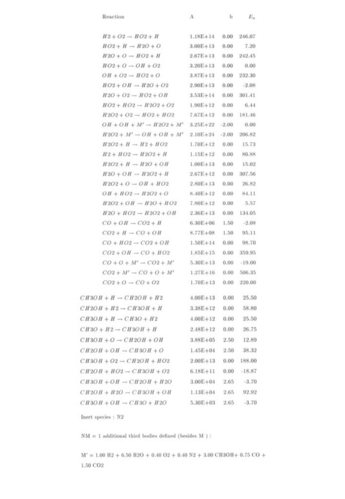
The chemical species participating in the methanol-air auto-ignition system include CH3OH, CH2OH, CH3O, CH2O, CHO, CO, CO2, O2, H2, H2O, H, O, OH, HO2, H2O2, CH4, CH3, CH2, CH, and N2. Denoting each species concentration to be an element of the species concentration vector y(t) enables the reaction rate equation to be expressed as
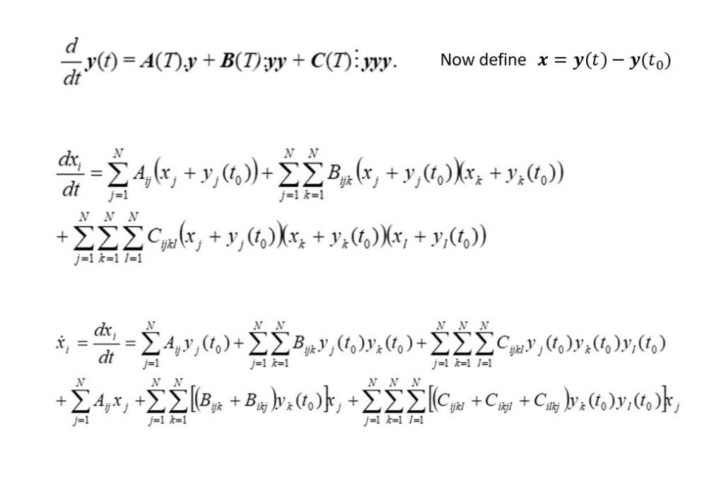
The top left equation in Figure 2 describes the rate of change of the species concentrations comprising the elements of the vector y(t). The right hand side of the equation contains 3 vector terms. The first term describes thermal decomposition reactions, the second term describes bi-molecular collision reactions, while the third term describes termolecular (3-body) collision reactions. If the solution is determined at t = t0, then the concentration displacement vector is defined to be x(t) = y(t) – y(t0). The second equation in Figure 2 is for the concentration displacement vector x(t), which is a non-linear equation containing x2 and x3 terms. The equation in x is linearised by retaining terms that are linear in x, and discarding the x2 and x3 terms, as seen in the bottom equation. This equation now has the form
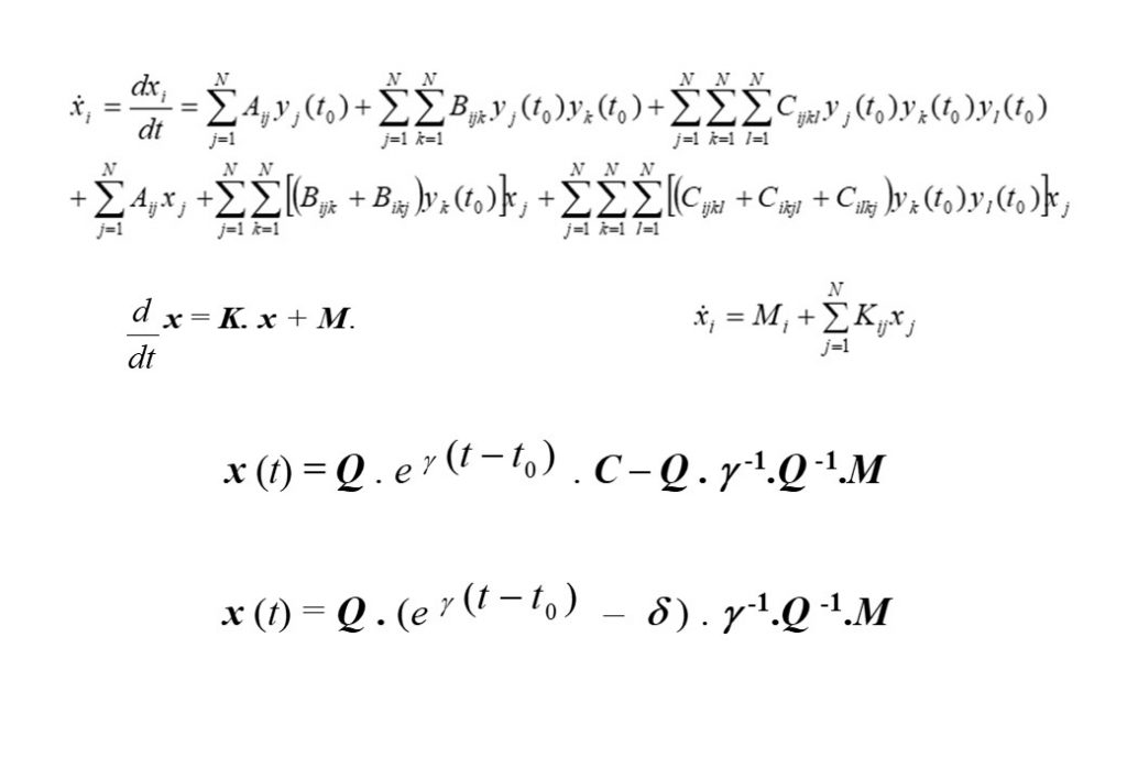
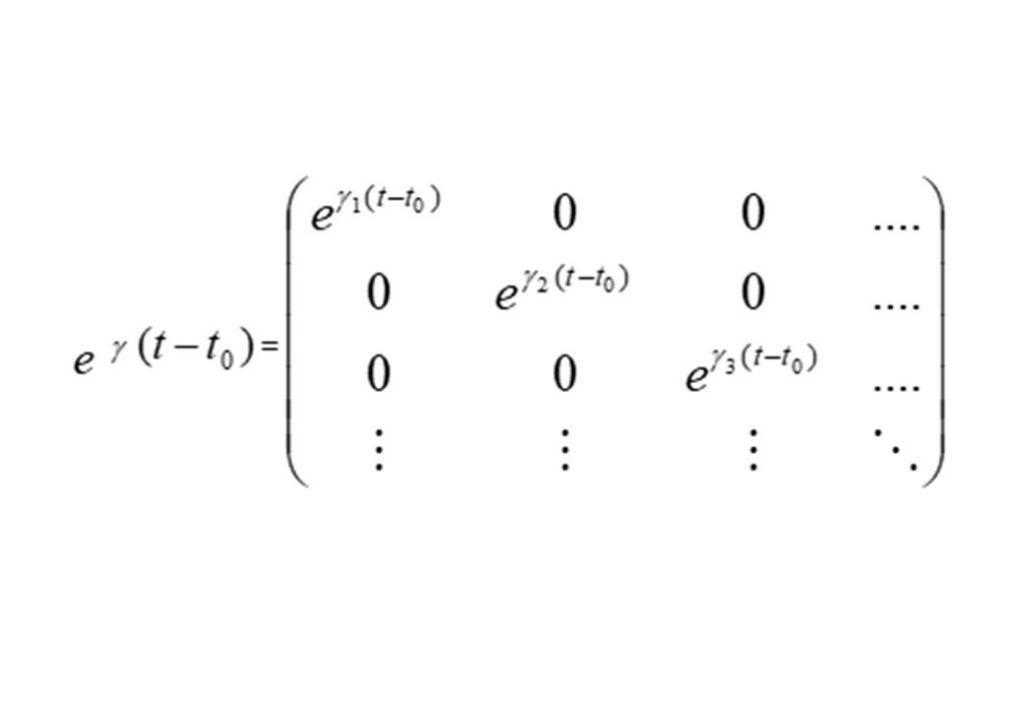
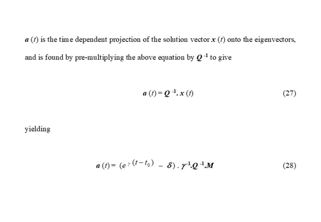
The analytic solution to this vector system of equations in x is given in the second to bottom equation. The application of the initial conditions x(0) = 0 permits the exact analytic solution to be obtained (bottom equation for x(t)), where Q is the matrix comprised of the independent eigenvectors of the K matrix, and δ the diagonal unit matrix. eγ(t-t0) is the diagonal matrix with diagonal matrix elements containing the eigenvalues of matrix K, given by
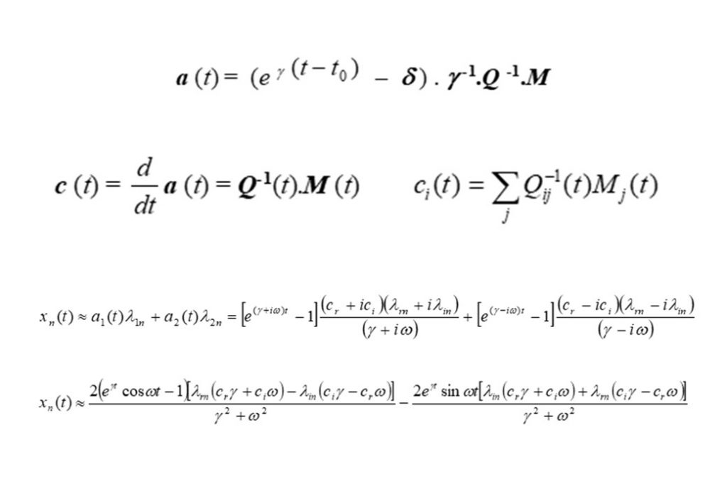
The second of the equations in Figure 6 show the projection of the eigenvectors (defined by matrix Q) onto the rate of reaction (defined by matrix M), thereby resolving the contribution made to dx/dt = M by each eigenvector at each point in time in the evolution of the auto-ignition system. The bottom two equation are the approximate solutions for x(t) based on two dominant eigenvectors forming a complex conjugate pair of eigenvectors.
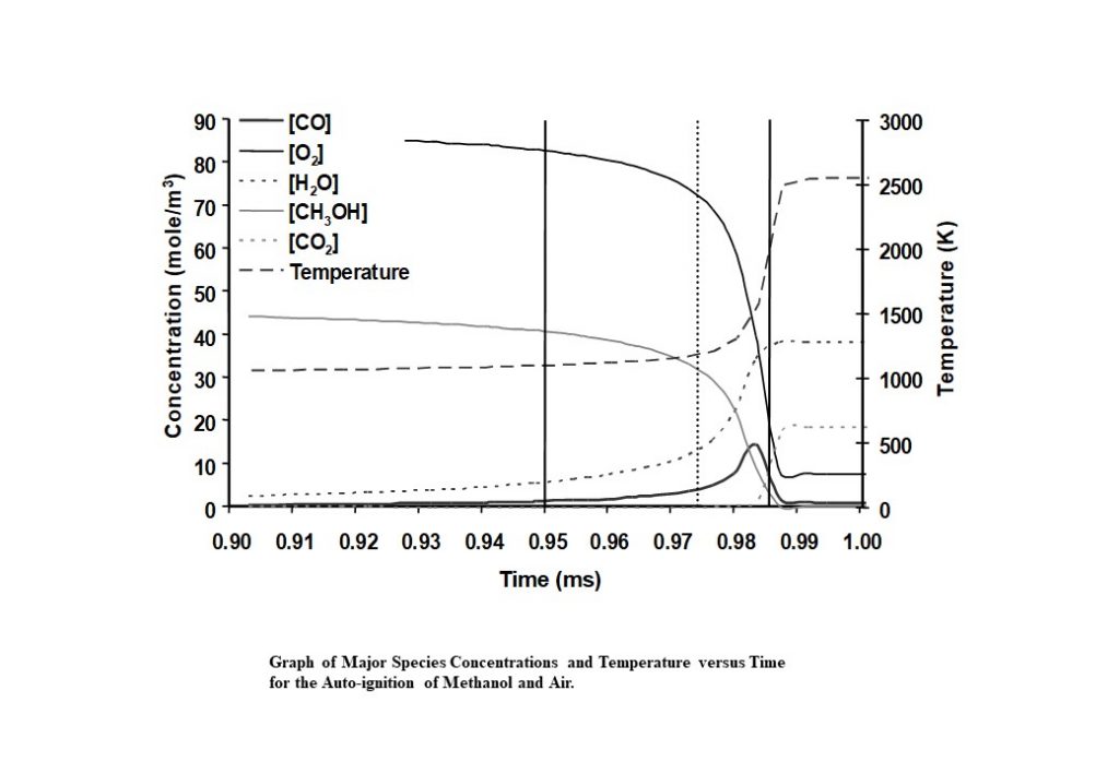
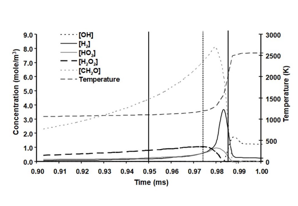
The system that is being modelled is based on pressure measurements taken from a knocking, naturally aspirated Ricardo E6 engine that was operating using methanol as engine fuel. Temperature measurements were obtained during the compression stroke using Coherent Anti-Stokes Raman Scattering (CARS) spectroscopy. Following spark ignition, the unburned methanol-air end-gas mixture was assumed to be adiabatically compressed by the piston and the flame. Hence the temperature profile was being driven by a combination of externally measured pressure and auto-ignition heat release. The integrated solution for the temperature and species concentrations y(t) was numerically integrated to yield the following graphs.
There are a number of interesting features in the eigenvectors and eigenvalues that control the evolution of the auto-ignition system. At least four eigenvectors have eigenvalues that are numerically zero, that reflect the conservation of nitrogen in the form of N2, and the elements carbon, hydrogen and oxygen (species C, H, and O). The dominant eigenvectors are given in Figures 8 – 12 below. The evolving solutions for y(t) are initially dominated by two real eigenvectors that have real, positive eigenvalues.
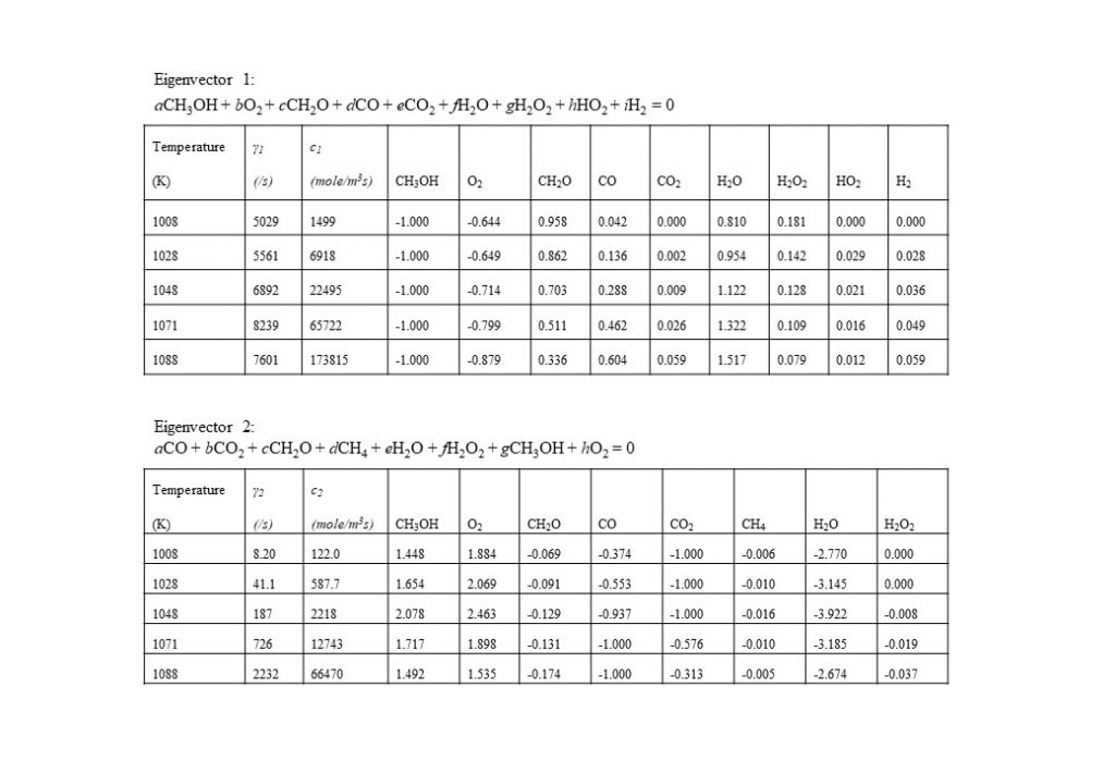
In the temperature range 1,000K < T < 1,090K, two real eigenvectors with positive eigenvalues dominate the solution for y(t). The first dominant eigenvector reflects the consumption of methanol (CH3OH) by oxygen (O2) to form water (H2O) and formaldehyde (CH2O). The second dominant eigenvector reflects reverse reactions that consume CH2O, CO and CO2, to form methanol (CH3OH) and oxygen (O2).
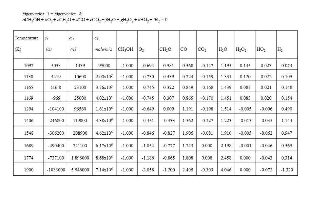
At a temperature of approximately 1,090K, the dominant real eigenvector solutions couple together to form a complex conjugate pair. This marks a point of inflection transition in the solution (bifurcation), when the dominant explosive modes couple together in a complex conjugate pair to form the initial period of an oscillatory solution. Note also that the real component of the eigenvalue γ changes sign from positive to negative at T = 1,166K. Figure 9 also shows the how the dominant set of eigenvectors, eigenvalues, species coefficients and eigenvector reaction rates vary with temperature in the temperature range 1,097K < T < 1,900K. As can be seen by the comparison of the magnitude of the eigenvector rates c1(1,774K) against c1(1,900K), this coupled eigenvector pair begin to diminish in importance relative to eigenvector 4 shown in Figure 10 below. This means that the dominant oxidation process shifts from methanol (CH3OH), oxygen (O2) and formaldehyde (CH2O) reacting to form carbon monoxide (CO) and water (H2O), to the oxidation of carbon monoxide (CO) and oxygen (O2), reacting to form carbon dioxide (CO2).
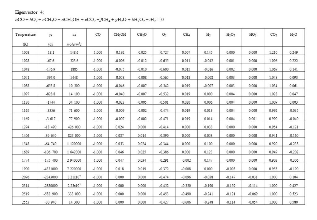
Figure 10 shows the next dominant eigenvector and eigenvalue that contributes to the integrated solution for the species concentration vector y(t). Eigenvector 4 shows the growth in importance with temperature of the conversion of carbon monoxide (CO) and oxygen (O2) to carbon dioxide (CO2). Note the increase in eigenvector resolved rate c4 in the temperature range 1,800K < T < 2,500K.
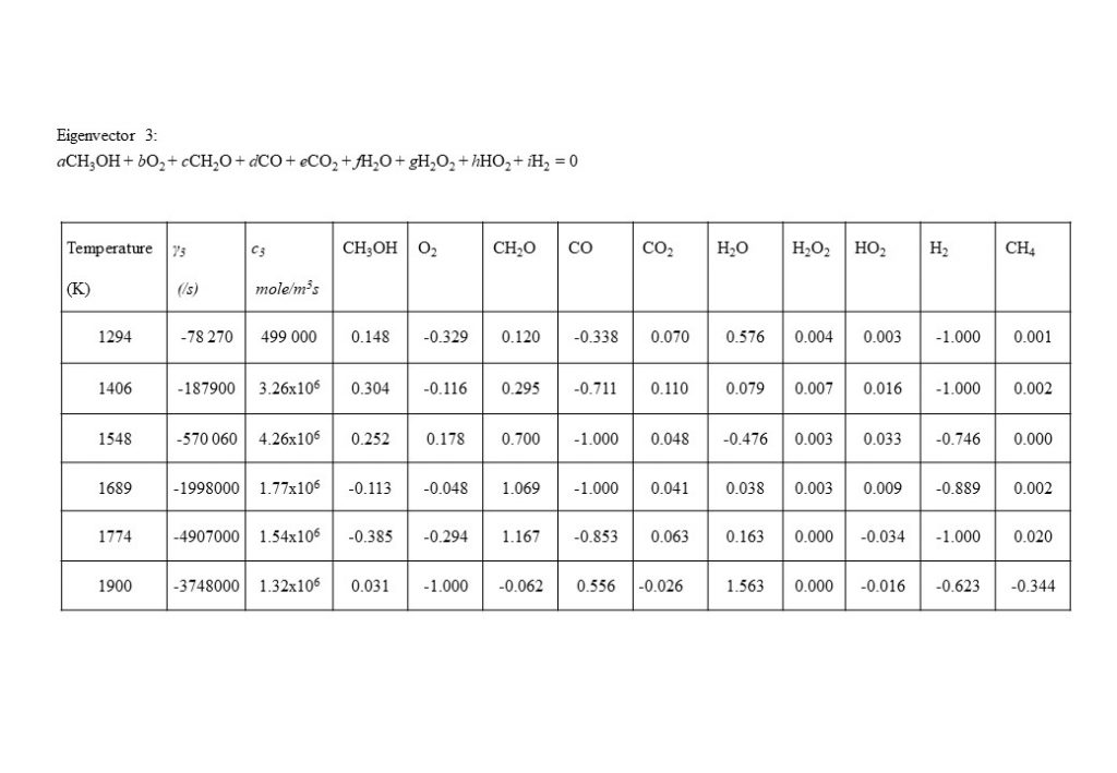
An important eigenvector contribution to the solution for y(t), with a rate value approximately an order of magnitude lower than for eigenvectors 1, 2 and 4, is the eigenvector that describes the consumption of molecular hydrogen (H2) and carbon monoxide (CO) to form formaldehyde (CH2O) (reverse reduction reaction to the dominant forward oxidation reactions) in the temperature range 1,300K < T < 1,900K.
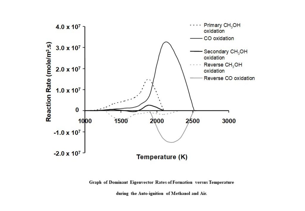
Figure 12 shows the contribution the eigenvectors and eigenvalues make to the formation and consumption of species involved in the methanol-air auto-ignition process. Each curve in the graph represents the eigenvector-specific rate of change of species concentration as a function of auto-ignition system temperature c(T). The black dashed line (representing complex conjugate eigenvectors 1 & 2) shows the eigenvector-related c1&2 increasing to a maximum at approx. 1,800K, and then decreasing to zero by 2,100K. This curve represents the main methanol oxidation route to form water (H2O), formaldehyde (CH2O) and carbon monoxide (CO). The solid black line represents eigenvector 4 above, with c4 gradually increasing to a maximum value at 2,100K, and then decreasing to zero at 2,550K. This curve represents the main carbon monoxide oxidation route to form carbon dioxide (CO2).
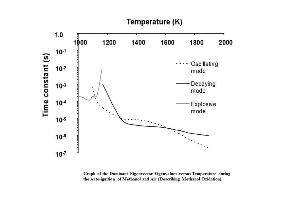
Figure 13 shows the real and imaginary parts of the eigenvalues corresponding to the eigenvectors that dominate the methanol oxidation process, as a function of the auto-ignition system temperature. Initially, for T < 1,090K, the dominant eigenvector has an eigenvalue that is real. However, at approx. 1,090K, the two dominant, real eigenvectors couple to become a complex conjugate pair with complex components and eigenvalues. The kink in the grey curve shows where this occurs. Once the two dominant eigenvectors are coupled, the real part of the eigenvalue is positive (grey curve). However, as the system evolves, the positive real part decreases until it passes zero to become negative (transitioning to the black curve in Figure 13). In the temperature regime 1,200K < T < 1,900K, the negative, real part of the complex eigenvalue continues to decrease, indicating that the methanol oxidation is tending to an equilibrium.
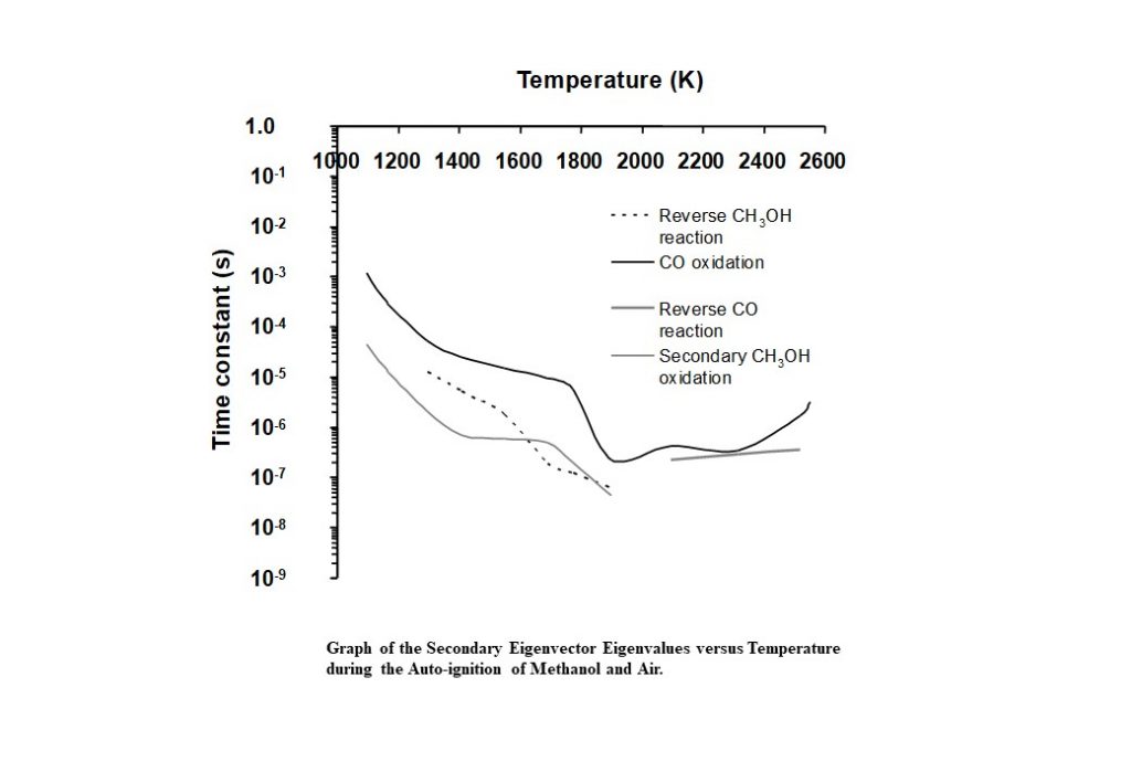
Figure 14 shows the eigenvalues that correspond to the eigenvectors that dominate the solution trajectory of the auto-ignition system, as a function of system temperature. Aside from complex, coupled eigenvectors 1 and 2, the dominant eigenvector here is eigenvector 4, and its eigenvalue is shown as the solid black line in Figure 14. The time constant decreases consistently in the temperature range 1,100K < T < 1,800K. However, in the temperature range of 1,800K – 2,000K, the time constant undergoes an alteration in its rate of change, decreases significantly, to achieve its minimum of 2.31 x 10⁻⁷s at 1,900K. This change in behaviour is prompted by the change in behaviour of the complex conjugate eigenvectors 1 and 2 and the corresponding eigenvalues and rates in the temperature range 1,800K – 1,900K. However, this eigenvector has an eigenvalue that begins to increase as the temperature rises to its equilibrium. This means that the reaction describing carbon monoxide oxidation to carbon dioxide has not equilibrated.